Mini-Project 03 - Visualizing and Maintaining the Green Canopy of NYC

Author

DolmaDev

Introduction

In this mini-project, I walk through the full process of using an API, handling a large geospatial dataset, and applying spatial analysis to understand patterns in NYC’s urban tree canopy. I rely on municipal open data—including the NYC Tree Points API and the City Council District shapefiles; and build a reproducible workflow that covers responsible data acquisition, paging through a large API, combining spatial data, and creating clear visualizations.

After exploring citywide trends, I focus on District 32 (South Queens), which stood out in my analysis with the highest proportion of dead trees in the city. Using what I learned from the spatial join and district-level comparisons, I developed a short, data-supported proposal for a targeted tree revitalization program. This helps show how open data and geospatial tools can support real municipal decision-making and how district-level insights can translate directly into policy recommendations.

Loading Libraries

Code

library(sf)

Linking to GEOS 3.13.0, GDAL 3.8.5, PROJ 9.5.1; sf_use_s2() is TRUE

Code

library(tidyverse)

── Attaching core tidyverse packages ──────────────────────── tidyverse 2.0.0 ──
✔ dplyr     1.1.4     ✔ readr     2.1.5
✔ forcats   1.0.1     ✔ stringr   1.6.0
✔ ggplot2   4.0.0     ✔ tibble    3.3.0
✔ lubridate 1.9.4     ✔ tidyr     1.3.1
✔ purrr     1.2.0

── Conflicts ────────────────────────────────────────── tidyverse_conflicts() ──
✖ dplyr::filter() masks stats::filter()
✖ dplyr::lag()    masks stats::lag()
ℹ Use the conflicted package (<http://conflicted.r-lib.org/>) to force all conflicts to become errors

Data Acquisition and Preparation

Task 1 — Council District Boundaries

Please find the data acquisition and preparation steps folded below:

Code

get_council_districts <- function() {

# Ensure data/mp03 directory exists
data_dir <- file.path("data", "mp03")
if (!dir.exists(data_dir)) {
dir.create(data_dir, recursive = TRUE, showWarnings = FALSE)
}

# File paths
zip_path <- file.path(data_dir, "nycc_25c.zip")
shp_dir  <- file.path(data_dir, "nycc_25c")
rds_path <- file.path(data_dir, "council_districts_wgs84.rds")

# Direct download URL
council_url <- "https://s-media.nyc.gov/agencies/dcp/assets/files/zip/data-tools/bytes/city-council/nycc_25c.zip"

# Download only if needed
if (!file.exists(zip_path)) {
download.file(url = council_url, destfile = zip_path, mode = "wb")
}

# Unzip only if needed
if (!dir.exists(shp_dir)) {
unzip(zip_path, exdir = data_dir)
}

# If processed version exists, return it
if (file.exists(rds_path)) {
return(readRDS(rds_path))
}

# Find the .shp file
shp_file <- list.files(
path       = shp_dir,
pattern    = "\\.shp$",
full.names = TRUE
)

if (length(shp_file) == 0) {
stop("No .shp file found in data/mp03/nycc_25c.")
}

# Read + transform to WGS84
districts_raw <- sf::st_read(shp_file[1], quiet = TRUE)
districts_wgs84 <- sf::st_transform(districts_raw, crs = "WGS84")

saveRDS(districts_wgs84, rds_path)
districts_wgs84
}

# Create council districts object for later use

districts <- get_council_districts()

Task 2 — NYC Tree Points via API (httr2)

Code

library(httr2)
get_tree_points <- function(limit = 10000, max_pages = Inf) {

data_dir <- file.path("data", "mp03")
if (!dir.exists(data_dir)) {
dir.create(data_dir, recursive = TRUE, showWarnings = FALSE)
}

# Cache file for the fully combined data

trees_rds <- file.path(
data_dir,
sprintf("treepoints_all_limit%05d.rds", limit)
)

# Only use cache when doing a full run (max_pages = Inf)

if (is.infinite(max_pages) && file.exists(trees_rds)) {
message("Loading cached tree points from RDS...")
return(readRDS(trees_rds))
}

# NYC OpenData Tree Points GeoJSON endpoint

base_url <- "https://data.cityofnewyork.us/resource/hn5i-inap.geojson"

sf_list <- list()
offset  <- 0L
page    <- 0L

repeat {
page <- page + 1L
if (page > max_pages) break  # safety for testing

# File name for this page (offset-based)
file_name <- sprintf("treepoints_limit%05d_%06d.geojson", limit, offset)
file_path <- file.path(data_dir, file_name)

# Only download if file not already present
if (!file.exists(file_path)) {
  message("Downloading page ", page, " (offset = ", offset, ")")
  
  req <- request(base_url) |>
    req_url_query(
      "$limit"  = limit,
      "$offset" = offset
    )
  
  resp <- req_perform(req)
  
  # Write raw bytes to file so sf::st_read can open it later
  writeBin(resp_body_raw(resp), file_path)
} else {
  message("Using existing file for page ", page, " (offset = ", offset, ")")
}

# Read the GeoJSON for this page
message("Reading ", file_path)
page_sf <- sf::st_read(file_path, quiet = TRUE)

n_rows <- nrow(page_sf)
if (n_rows == 0) {
  message("No rows in this page; stopping.")
  break
}

sf_list[[length(sf_list) + 1L]] <- page_sf

# If fewer than limit rows, we've reached the end
if (n_rows < limit) {
  message("Last page (", n_rows, " rows < limit ", limit, "); stopping.")
  break
}

# Otherwise, move offset forward and continue
offset <- offset + limit

}

if (length(sf_list) == 0) {
stop("No tree data downloaded or read. Check the API URL or parameters.")
}

# Combine all pages into one big sf object

trees_sf <- do.call(rbind, sf_list)

# Cache full results only when doing a full run

if (is.infinite(max_pages)) {
saveRDS(trees_sf, trees_rds)
}

trees_sf
}

Download full tree data

Code

trees <- get_tree_points(limit = 5000)

Loading cached tree points from RDS...

Exploratory Analysis

Task 3 prep — Sample Tree Data for Mapping

Code

set.seed(9750)  # for reproducibility

trees_small <- dplyr::slice_sample(trees, n = 10000)

Mapping NYC Trees

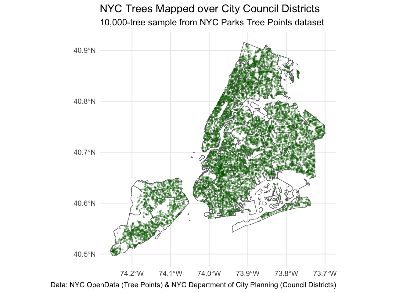
Task 3 — Plot All Tree Points over Council Districts

Code

library(ggplot2)

ggplot() +

# Layer 1: Council district boundaries

geom_sf(
data  = districts,
fill  = "white",
color = "grey40",
linewidth = 0.3
) +

# Layer 2: Tree points (sample)

geom_sf(
data  = trees_small,
color = "darkgreen",
alpha = 0.3,
size  = 0.4
) +

coord_sf() +

labs(
title    = "NYC Trees Mapped over City Council Districts",
subtitle = "10,000-tree sample from NYC Parks Tree Points dataset",
caption  = "Data: NYC OpenData (Tree Points) & NYC Department of City Planning (Council Districts)"
) +

theme_minimal()

District-Level Analyses of Trees

Task 4— Join Trees to Council Districts

Code

library(dplyr)
library(sf)

# Spatial join: each tree gets its council district attributes

trees_joined <- st_join(
  trees,
  districts,
  join = st_intersects,
  left = TRUE 
)

1. District with Most Trees

District 51 has the highest total number of trees in NYC, with approximately 70,965 trees recorded—the largest count of any council district.

Code

trees_by_district <- trees_joined |>
  st_drop_geometry() |>
  group_by(CounDist) |>
  summarise(n_trees = n(), .groups = "drop") |>
  arrange(desc(n_trees))

head(trees_by_district, 5)

# A tibble: 5 × 2
  CounDist n_trees
     <int>   <int>
1       51   70965
2       50   52500
3       19   49940
4       23   44917
5       13   36665

2. District with Highest Tree Density

District 7 has the highest tree density in New York City, with roughly 0.000284 trees per square meter, indicating the densest canopy relative to land area.

Code

trees_density <- trees_joined |>
  st_drop_geometry() |>
  group_by(CounDist, Shape_Area) |>
  summarise(n_trees = n(), .groups = "drop") |>
  mutate(tree_density = n_trees / Shape_Area) |>
  arrange(desc(tree_density))

head(trees_density, 5)

# A tibble: 5 × 4
  CounDist Shape_Area n_trees tree_density
     <int>      <dbl>   <int>        <dbl>
1        7  55186140.   15648     0.000284
2       39 118294553.   32403     0.000274
3        2  48322121.   11563     0.000239
4        9  56263769.   13455     0.000239
5        5  37752246.    8326     0.000221

3. District with Highest Fraction of Dead Trees

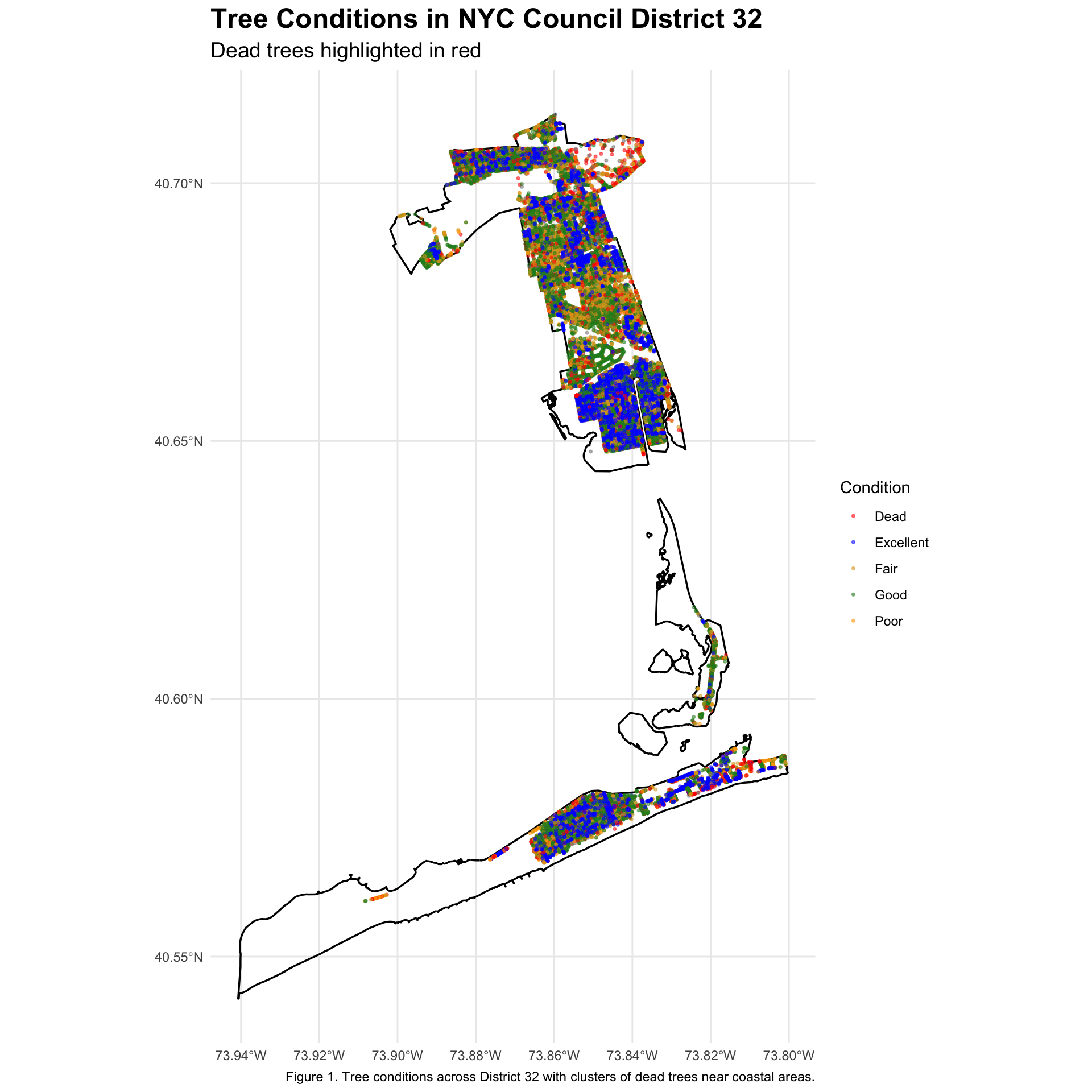
District 32 has the highest proportion of dead trees, with 14.3% of all tree records in the district classified as dead, suggesting elevated maintenance needs.

Code

dead_fraction <- trees_joined |>
  st_drop_geometry() |>
  mutate(is_dead = tpcondition == "Dead") |>
  group_by(CounDist) |>
  summarise(
  n_trees      = n(),
  n_dead       = sum(is_dead, na.rm = TRUE),
  frac_dead    = n_dead / n_trees,
  .groups = "drop"
) |>
arrange(desc(frac_dead))

head(dead_fraction, 5)

# A tibble: 5 × 4
  CounDist n_trees n_dead frac_dead
     <int>   <int>  <int>     <dbl>
1       32   30270   4315     0.143
2       30   23012   3231     0.140
3        2   11563   1576     0.136
4       50   52500   7087     0.135
5       29   19994   2688     0.134

4. Most Common Species in Manhattan

The Thornless Honeylocust (Gleditsia triacanthos var. inermis) is the most common tree species in Manhattan, with over 17,000 individuals city-recorded.

Code

# Add Borough Labels

trees_with_boro <- trees_joined |>
  mutate(
    borough = case_when(
      CounDist >=  1 & CounDist <= 10 ~ "Manhattan",
      CounDist >= 11 & CounDist <= 18 ~ "Bronx",
      CounDist >= 19 & CounDist <= 32 ~ "Queens",
      CounDist >= 33 & CounDist <= 48 ~ "Brooklyn",
      CounDist >= 49 & CounDist <= 51 ~ "Staten Island",
      TRUE ~ NA_character_
      )
  )

manhattan_species <- trees_with_boro |>
  st_drop_geometry() |>
  filter(borough == "Manhattan", !is.na(genusspecies)) |>
  group_by(genusspecies) |>
  summarise(n_trees = n(), .groups = "drop") |>
  arrange(desc(n_trees))

head(manhattan_species, 5)

# A tibble: 5 × 2
  genusspecies                                               n_trees
  <chr>                                                        <int>
1 Gleditsia triacanthos var. inermis - Thornless honeylocust   17310
2 Platanus x acerifolia - London planetree                     11593
3 Pyrus calleryana - Callery pear                               8793
4 Quercus palustris - pin oak                                   8107
5 Ginkgo biloba - maidenhair tree                               7462

5. Tree Closest to Baruch College

The tree closest to Baruch College is a Sweetgum (Liquidambar styraciflua) located in District 2 and reported to be in good condition.

Code

new_st_point <- function(lat, lon){
st_sfc(st_point(c(lon, lat)), crs = "WGS84")
}

baruch_point <- new_st_point(lat = 40.7403, lon = -73.9833)

closest_tree <- trees_joined |>
mutate(distance_to_baruch = st_distance(geometry, baruch_point)) |>
slice_min(distance_to_baruch, n = 1)

closest_tree |>
st_drop_geometry() |>
select(CounDist, genusspecies, tpcondition, distance_to_baruch)

  CounDist                       genusspecies tpcondition distance_to_baruch
1        2 Liquidambar styraciflua - sweetgum        Good       19.48124 [m]

Government Project Design: NYC Parks Proposal

Revitalizing the Urban Canopy in District 32 (South Queens)

As the office of the City Council representative for District 32, we propose a Tree Replacement and Canopy Revitalization Program aimed at improving tree health, public safety, and long-term climate resilience across South Queens. District 32 includes coastal neighborhoods such as Howard Beach, Ozone Park, Rockaway Beach, and Broad Channel—areas that have historically faced storm damage, high winds, and saltwater exposure. These environmental stressors have contributed to elevated tree mortality, creating safety hazards and reducing canopy coverage in vulnerable communities.

Our analysis of NYC Parks Tree Points data shows that District 32 has the highest proportion of dead trees in New York City. Approximately 4,315 trees (14.3%) in the district are classified as dead—substantially higher than comparable districts including District 30 (14.0%), District 2 (13.6%), and District 50 (13.5%). This pattern of decline highlights an urgent need for targeted restoration and proactive investment in tree health.

Project Scope

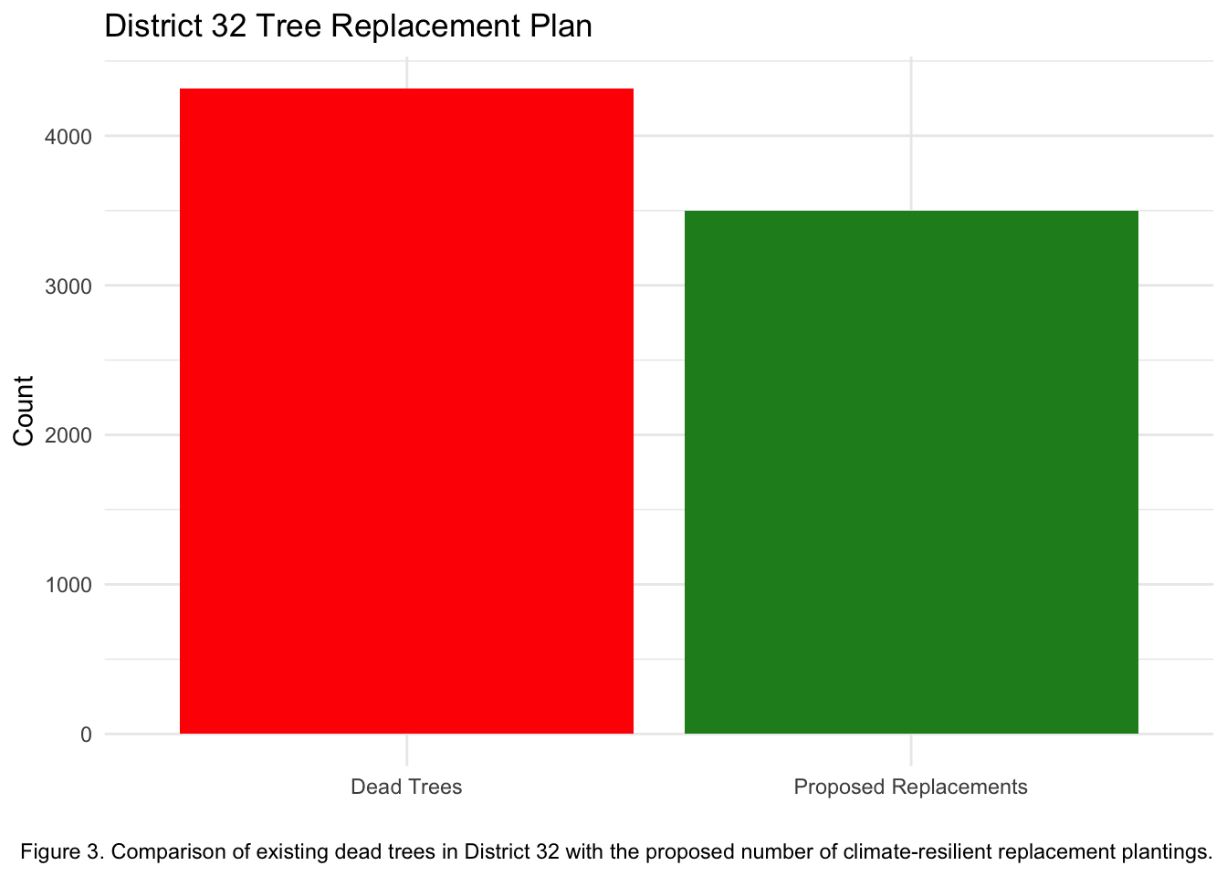
The proposed program includes: - Removal of 4,000+ dead or hazardous trees across the district
- Planting of 3,500 new, climate-resilient street trees, emphasizing coastal-adapted species
- Restoration of approximately 2,500 planting sites through stump removal
- Ongoing monitoring and maintenance for the first three years after planting

Why District 32?

Compared with tree-dense districts like District 7, highly populated canopy districts like District 19, or the large-area forested District 51, District 32 stands out due to its combination of moderate canopy coverage and the highest mortality burden citywide. This creates an opportunity for meaningful canopy revitalization that supports both environmental equity and public safety.

Conclusion

District 32’s high mortality burden, combined with its exposure to severe weather and environmental stressors, makes it a clear priority for targeted investment. This Tree Replacement and Canopy Revitalization Program strengthens community safety, restores lost greenery, enhances environmental resilience, and ensures more equitable access to the environmental benefits of NYC’s urban forest.

Visual Evidence

Figure 1. Tree Conditions in District 32

Code

trees_d32 <- trees_joined |> dplyr::filter(CounDist == 32)
district_32 <- districts |> dplyr::filter(CounDist == 32)

ggplot() +
  geom_sf(data = district_32, fill = NA, color = "black", size = 0.6) +
  geom_sf(data = trees_d32, aes(color = tpcondition), alpha = 0.5, size = 0.6) +
  scale_color_manual(values = c(
    "Dead" = "red",
    "Good" = "forestgreen",
    "Poor" = "orange",
    "Excellent" = "blue",
    "Fair" = "goldenrod"
  )) +
  labs(
    title = "Tree Conditions in NYC Council District 32",
    subtitle = "Dead trees highlighted in red",
    color = "Condition",
    caption = "Figure 1. Tree conditions across District 32 with clusters of dead trees near coastal areas."
  ) +
  theme_minimal() +
  theme(
    plot.title = element_text(size = 18, face = "bold"),
    plot.subtitle = element_text(size = 14),
    legend.position = "right"
  )

Figure 2. Fraction of Dead Trees: District 32 vs. Comparable Districts

Code

compare_dead <- dead_fraction |>
dplyr::filter(CounDist %in% c(32, 30, 2, 50))

ggplot(compare_dead, aes(x = factor(CounDist), y = frac_dead)) +
  geom_col(fill = "firebrick") +
  labs(
  title = "Fraction of Dead Trees by District",
  x = "District",
  y = "Fraction Dead",
  caption = "Figure 2. District 32 leads the city in tree mortality, with a higher   proportion of dead trees than Districts 30, 2, and 50."
  ) +
  theme_minimal()

Figure 3. Proposed Replacement Plan for District 32

Code

ggplot(compare_dead |> dplyr::filter(CounDist == 32)) +
  geom_col(aes(x = "Dead Trees", y = n_dead), fill = "red") +
  geom_col(aes(x = "Proposed Replacements", y = 3500), fill = "forestgreen") +
  labs(
  title = "District 32 Tree Replacement Plan",
  x = "",
  y = "Count",
  caption = "Figure 3. Comparison of existing dead trees in District 32 with the proposed number of climate-resilient replacement plantings."
  ) +
  theme_minimal()

This work ©2025 by DolmaDev was initially prepared as a Mini-Project for STA 9750 at Baruch College. More details about this course can be found at the course site and instructions for this assignment can be found at MP #03